Tutorial: How to perform a transient thermal analysis in SolidWorks

David Lane

8 Jun, 2013 03:40 PM

This is a tutorial for the 'Software Tricks of the Trade' Challenge found here http://grabcad.com/challenges/software-tricks-of-the-trade

Note: This is CPU intensive.

You can view the tutorial files on GrabCad here: Tutorial: How to perform a transient thermal analysis in SolidWorks

The ZIP files contains the parts and assembly that I used to create this tutorial as well as some addition images that may help you find commands within SolidWorks. It also has the analysis saved. You can download it from the project link or you can additionally download the attached ZIP file, directly from here.

A thermal analysis can be used to study the effects that temperature has on components or assemblies. Using a transient analysis can show you how the temperature varies with time. This tutorial will help you understand the basics of performing a transient thermal analysis in SolidWorks. Knowledge of heat transfer is preferable when doing a study like this.

1. Step 1:

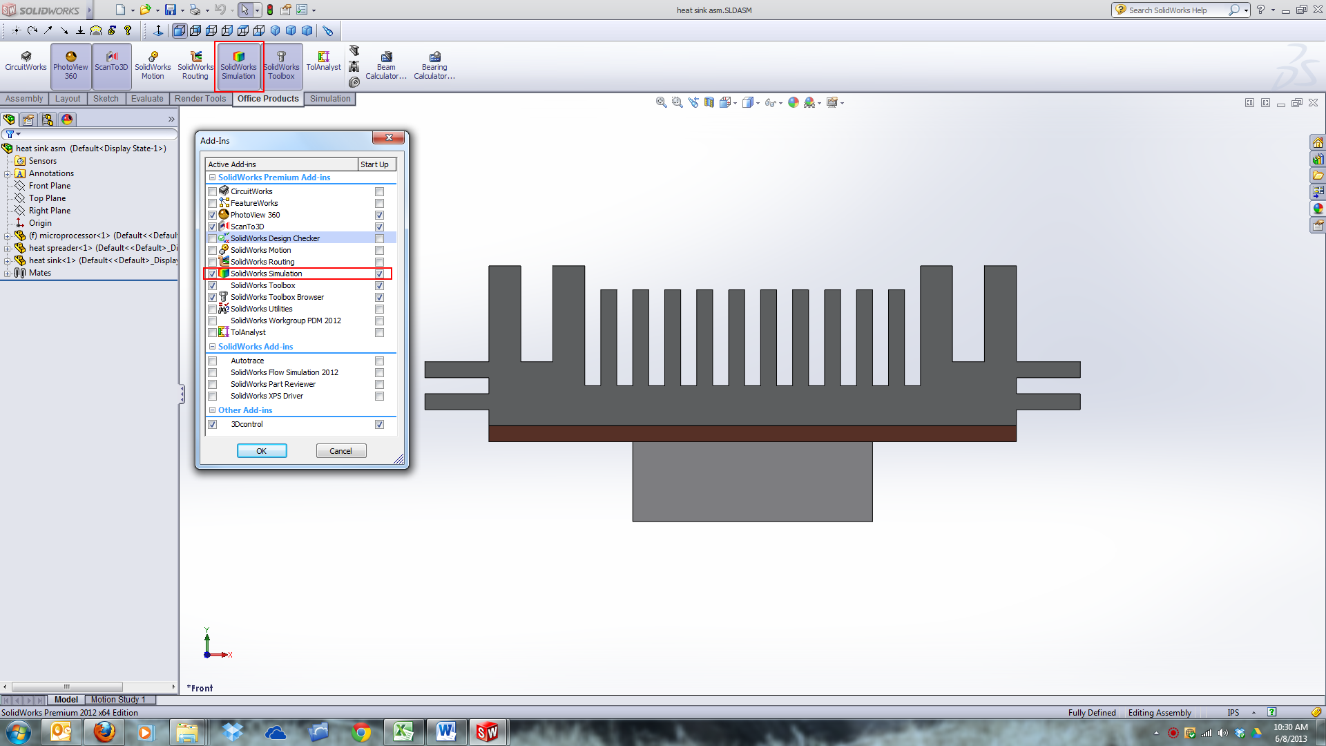
   Open the part or assembly you want to perform the study on. Make sure materials are applied to each component. You will also need to turn on the ‘’SolidWorks Simulation’ add in. To this click the ‘Office Products’ tab and click ‘SolidWorks Simulation.’ Alternatively you can click ‘Tools’ from the menu bar and then click ‘Add Ins…’ and check ‘SolidWorks Simulation’ on the left side. If you check it on the right side it will not be active; though it will load when SolidWorks is started. Once you have activated the add in go to the new ‘Simulation Tab and click the down arrow beneath ‘Study Advisor’ followed by ‘New Study’
   

   

2. Step 2:

   Now you can name your study if you choose to. In addition you will want to select ‘Thermal’ for the study type. Then click the green check mark. Next right click the study name at the top of the tree and select ‘Properties.’ Now select transient and modify the settings as needed. You may select the total time as well as the increments to run the analysis. We will use ‘600 sec’ for the total time and ‘180 sec’ for the time increment. This will perform the studies only at those time increments and will allow us to enter an initial temperature of the components.
   Note: That I named my study ‘Stead State’ though it should be named ‘Transient.’

   

3. Step 3:

   Now you will need to apply the ‘Thermal Loads.’ This can be accomplished by right clicking ‘Thermal Loads’ and selecting the necessary load types. For this example there will be ‘Heat Power,’ ‘Convection,’ and ‘Temperature.’
   Because this is a heat sink which captures heat from, typically, a microprocessor you will need to select ‘Heat Power’ and select the entire ‘microprocessor’ part. To select the ‘microprocessor’ you will need to select it from the model tree. If you try to select it by clicking one of the faces it will not select it correctly. I entered ‘5 W’ for the amount of heat power in this example.
   

   

4. Step 4:

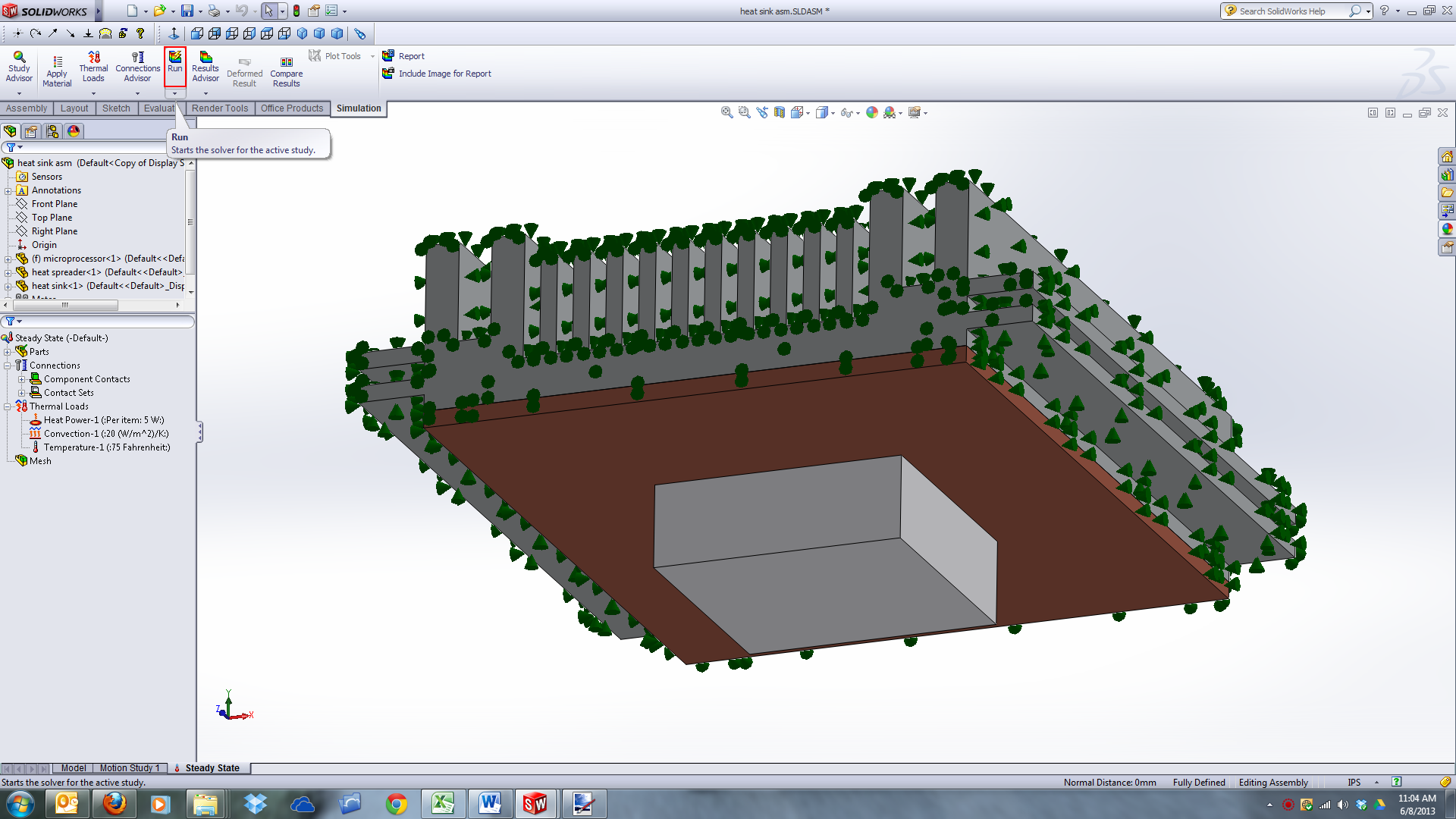
   In addition to heat power, the heat sink is also exposed to convection. Now right click ‘Thermal Loads’ and select ‘Convection.’ This will be almost the same as ‘Heat Power’ except we will need to select all faces except for the bottom faces that are not exposed to convection. To do this simply click ‘Select all exposed faces’ then hold down the ‘CTRL’ key and click the faces marked in the image below to deselect them. I will use ‘20 (W/m^2)/K’ for this example because a fan would typically be blowing air over the heat sink. Additionally I will set the ambient temperature to ‘300 K.’
   

   

5. Step 5:

   Now we need to apply the initial temperature. This can be done by right clicking the ‘Thermal Loads’ and clicking ‘Temperature.’ Next select ‘Initial Temperature.’ You also need to select the parts from the model tree, as before, that you want to have this initial temperature. For our example all three parts will be selected with an initial temperature of ’75 Fahrenheit.’
   

   

6. Step 6:

   We now need to establish contact sets. The contact sets for this assembly are between the heat spreader and the microprocessor. To apply the contact set, right click ‘Connections’ and then click ‘Contact Set.’ Select the faces as shown in the image below. For this example we will use a distributed thermal resistance of ‘0.0002 (K-m^2)/W.’
   

   

7. Step 7:

   Click ‘Run.’ This will automatically create a mesh and run the analysis. You can additionally create a mesh prior to clicking run to adjust it to your liking with mesh controls. For starters it is easiest to just click ‘Run.’
   

   

8. Step 8:

   Next, analyze the data.
   

   

9. Step 9:

   By clicking the down arrow for ‘Results Advisor’ followed by ‘New Plot’ and ‘Thermal’ you can create a new plot for any of the steps you set up in the properties earlier or you can plot across all steps showing the maximum or minimum temperature.