

How to Make GrabCAD Voxel Print Slices Using Matlab

This tutorial is intended for users who already have a passing familiarity with Matlab and J750 operation.
It is NOT intended to be a comprehensive lesson on how to use the Matlab software or PolyJet printers.
The following is brought to you by Stratasys:
-
Step 1: What is Voxel?
Just like 2D digital images are made up of pixels, you can think of 3D digital shapes as being made up of “voxels.”
They are regular, rectangular structures that contain color or material data for that point in the 3D print.


In 3D: Voxelize In 2D Rasterize
But instead of picturing voxels in 3D, a better mental image may be thinking of what is happening in 2D, with every slice of a 3D print. Instead of shapes being “voxelized,” slices are being “rasterized.” You can see that to represent a letter in 2D, we have to make many decisions about which square in the grid is darkly filled, lightly filled, or not filled at all.
Because making thousands of those decisions for every slice results in a huge matrix of values, that is one reason to use Matlab, which has many tools to manipulate large matrices.

-
Step 2: General Slice Guidelines
It’s easy to imagine that if you had 1,000+ progressive slices for each layer of your voxel print that looked like this:

You could stack them one on top of each other in a J750 and get a print like this:

But there are some rules to follow.
-
Step 3: Rule 1: All slices must be the same dimensions
Every slice in our Voxel print must have the same pixel dimensions (width and height). For example, in our sphere below, each PNG slice is a rectangle 709 pixels high x 1424 pixels wide (even at slices near the top and bottom of the sphere, where not much is happening).
Those are just the dimensions the engineer who created the slices chose. He could have chosen any dimension, as long as EVERY slice in a print was the same.
We will use Matlab looping commands to make sure each slice is the same size.

-
Step 4: Rule 2: The Z gap between slices should match a printer layer setting
You should plan to slice your desired final shape at a layer height that matches what the J750 can do.
For example, in our sphere below, each PNG slice is assumed to be 0.027 mm from the next to make the final shape.

For reference, J750 layer heights are:

(Note: If your slice thickness does not match the printer layer thickness, the printer will try to compensate for the difference. For example, if you generate the slice thickness at 0.0135 mm, and your printing mode is High Mix, the printer will print each image twice to reach the desired thickness of 0.027 mm. Best practice is to create your slices to match the mode you will be printing in.
-
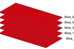
Step 5: Rule 3: All slices should be named sequentially using the same prefix
The Voxel Print utility does not know the “right” order for the slices. It simply goes by the file name.
It will look in a single folder and sequence all PNG files labeled with a defined prefix.
In this example, the prefix is “slice_”.
The sequence will be by increasing number.
We will use Matlab loops to sequentially number our slices as they are generated.

-
Step 6: Rule 4: Use only 6 RGB colors in all slices
The J750 can only hold 6 materials + support.
The Voxel Print Utility will separate material usage in each slice by RGB value.
Therefore, you can only use 6 RGB values in a given print, in all your slices combined.
For reference, here are the RGB values of some common J750 materials:


From here on, we will be getting into Matlab commands.
-
Step 7: Now, how is an RGB image stored in Matlab?
One of the sample images that comes with Matlab is ‘peppers.png’ (below).

To load that image into a Matlab variable, use the command:

After running that command, Matlab shows you that RGBsample is now defined as a 384 x 512 x 3 matrix:

To see any given pixel in peppers.png, use the command:

Results in:

That means that, 50 rows down and 100 columns over from the top corner of our peppers picture, there is a pixel with the RGB value of (66,38,68), or something like this:

-
Step 8: The simplest possible voxel print (a red brick)
Now we will attempt to make one of the simplest possible Voxel Prints, a uniform red brick:

To do so, we will use Matlab to define and number our required slices (not all slices shown).
Starting with the command:

Should result in a 300 x 600 x 3 matrix of integers:

Filled with zeros:

Now let’s make the first layer of the matrix = 161, the second layer = 35, and the third layer = 99. This corresponds to RGB of (161,35,99), which should be VeroMagenta.
>>brickslice(:,:,1) =161;
>>brickslice(:,:,2) =35;
>>brickslice(:,:,3) =99;
And then we test things with the Image Show (‘imshow’) command:
>>imshow(brickslice)
Which should lead to:

-
Step 9: A ‘for’ loop to sequentially number and name our 941 slices
General structure of a Matlab loop:

Our loop:

-
Step 10: Thoughts on the results of our first ‘for’ loop
If you saved that for loop in a Matlab ‘.m’ file and ran it, you might notice a few things:
Why did we specify 941 slices?If you remember, we wanted a brick that was 1 inch tall:

If our J750 is set to High Mix mode, slices are 0.027 mm apart, so 25.4 / 0.027 = 940.7, which I rounded to 941.
2. Why did all the resulting PNGs have the wrong dimensions?
If you right click on any PNG we just created and look at the “Properties,” you will see that they are not the 300x600 pixels we wanted:

This is because the Matlab ‘imshow’ command displays images at a default solution, which we must now change. We will show how to do this in the next step.
-
Step 11: Controlling output pixel dimensions in our ‘for’ loop
Our REVISED loop:

-
Step 12: Results of the Matlab slicing
In the same folder as your Matlab ‘.m’ file, you should now have 941 separate PNG slice files, all sequentially numbered and with the same prefix:

(I changed mine to ‘brick_slice’ to match the name of the .m file, you can set whatever prefix you want inside your loop.)

They should all have the correct pixel dimensions.
Now we are ready to move into GrabCAD Print
From here on, we will be using GrabCAD Print and the Voxel Utility
-
Step 13: The Voxel Print Utility will be found under “Apps” similar to Insight

-
Step 14: The Voxel Print Utility will open with this window


-
Step 15: Using the Voxel Print utility


-
Step 16: After hitting “Next” the utility runs

This is also the screen where errors would be shown. If you get the “Too Many Colors” error, see the Troubleshooting guide later in this presentation.
-
Step 17: Next we must map RGB values to J750 materials
This is where the Utility tells us which RGB values (up to 6, remember) it has found in our slices.
We must designate some J750 material to each value.

But see something wrong?
-
Step 18: Troubleshooting: the “Too many colors” error
Remember that we can only have 6 RGB values in our slices. But we only designated 1 in Matlab, so what gives? The answer comes from zooming into any PNG output from Matlab:
While the slices may look good in preview:

And even look good when you open one:

If you zoom in on a corner, you see the problem: DITHERING

This seems to be a default with how Matlab outputs images, that it tries to “Anti-alias” the edges of a solid color.
Better Matlab users than I may know the command to turn this off, but for now, be aware that if you designated 6 colors in your slice matrix, the Voxel Print utility will see these edges as EXTRA colors and give you an error, since they are new RGB values.
Photo editing software is a good way to check for this.
1. Turn on your color picker.
2. Click in the dithered area in your slice.
3. See if the RGB values are changing or different from what you intended.

If so, these extra RGB values are what is probably causing your “Too many colors” error!
Other options:
A. You have not designated the correct color as “background.”
B. Different alpha channels under colors are treated as different RGB values, so it’s really RGBA we can only have 6 of.
-
Step 19: Next we must map RGB values to J750 materials
Since we cannot fix the Matlab dithering issue now, we will designate a material to each found RGB value (I choose Yellow for the dither, hopefully that shouldn’t affect much):

-
Step 20: Hit “Finish” and the GCVF file should be created

-
Step 21: Before you add the GCVF file to your tray
You must turn on these two “Preferences” to be able to import a GCVF into GrabCAD Print:

And then you can import your GCVF file onto a tray.
-
Step 22: And we finally have our magenta cube
Wait? A cube?

I thought we were making a RECTANGLE, 300 pixels tall and 600 pixels wide?
This happened because… (see next step)
-
Step 23: X and Y directions have different DPI on a J750
Back in the Voxel Utility, you may have noticed these two non editable fields in the window.

Due to the nature of polyjet technology, pixels are stacked twice as tightly in the X direction as in the Y:

-
Step 24: This is why we got a 1 inch by 1 inch cube as our result
How do we know it is a 1 inch by 1 inch cube?
Because, if you add a CAD part which has cutouts every inch and every centimeter (which you should all have), you can see that the cube fits nicely between two “inch” cutouts.

(This is why I choose 300 x 600 in our original dimensions, so this would happen.)
-
Step 25: Conclusion
You may have noticed a few things during this process:
The preview does not display in color.

Just this little cube has 941 slices in it. To try and show those thousands of pixels for each of those 941 slices would crash most graphics cards. Which is why it is a simple gray preview for any .gcvf file.
2. We tried to create a red brick. The result was a magenta cube.

There is no “VeroRed.” In voxel printing, you will need to put a mix of J750 material-colored RGB voxels next to each other to get a certain color effect from a distance, like a TV does.
Also, be aware of the 300 DPI vs. 600 DPI issue when sizing.
3. Every single slice was the same

In this example, we used a Matlab ‘for’ loop to number our slices, using the same matrix every loop. But to realize the real power of Voxel printing, you will obviously want each slice to be unique, with the shape and materials and arrangement of voxels changing every single layer.
Programming that is beyond the scope of this tutorial, but there are many, many Matlab help documents detailing how to program your ‘for’ loops for ever increasing complexity. But this should be enough to get you started with Voxel Printing, and if you need any further assistance, contact your local Stratasys reseller or print@grabcad.com!
